A simulated AGILE observation

A good knowledge of the diffuse emission model is important also for sources analysis. In order to test the performances of our model from this point of view, we have simulated a set of ten AGILE observations with photons energy above 100 MeV of the second quadrant sky region for a total observing time of about 5 months. In these simulations we have included the diffuse emission model, the point sources from third EGRET catalog and a component of noise due to residual particle background. We have chosen 2GC 135+1 as test source for our analysis. 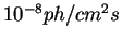The assumed flux is $10^{-6}$ photons per $cm^2$ per second above 100 MeV.
We performed two maximum likelihood analysis [Chen et al., 2004] on the test source using the AGILE and the EGRET models.

Table 3.1: Results of ALIKE analysis for the two models

Parameter (unit)	Value
2GC 135+01	Flux ( $10^{-8} ph/cm^2 s$)	G mult	G bias
EGRET model	179$\pm$5	0.271	11.1
AGILE model	149$\pm$5	0.789	7.85

Table 3.6 summarizes the results of the analysis. Second column represents the estimated flux of the test source. We found a better agreement with the simulated value using the AGILE model. Two more parameters are provided by the maximum likelihood method, the multiplicative (G-mult) and additive (G-bias) terms which allow the diffuse emission model used to better fit to the simulation. Also in this case we can notice that a smaller correction is needed for the AGILE model.

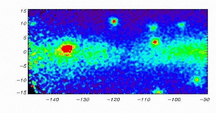
Figure 3.22: The AGILE (simulated) observations of the Galactic plane near 2CG 135+01, for energy $>$ 100 MeV, composed of ten AGILE pointing of the second quadrant sky region for a total observing time of about 5 months. with photons energy above 100 MeV. A component of noise due to residual particle background is also present in the simulation.