Next: New vs old model Up: Observing the Diffuse Emission Previous: Observing the Diffuse Emission Contents

The gamma-ray sky

The intensity of the diffuse gamma-ray flux (E

100 MeV) from different sky direction, M(l,b), foreseen by this model can be evaluated by:

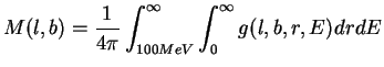$\displaystyle M(l,b) = \frac{1}{4 \pi} \int_{100 MeV}^\infty \int_0^\infty g (l,b,r,E) dr dE$

(3.1)

Figure 3.1 and 3.5 show the total AGILE model for the first and second Galactic quadrant. The contributions to the total emission produced by the different cosmic-rays targets, for the first Galactic quadrant, are shown in figure 3.2, 3.3 and 3.4 and are obtained respectively by substituting

in eq.3.1 with :

$\displaystyle g_{HI} = (q_{pp}+q_{br}) n_{HI}$

$\displaystyle g_{H2} = (q_{pp}+q_{br}) n_{H2}$

$\displaystyle g_{iC} = q_{iC} n_{ph}$

Figures 3.6, 3.7 and 3.8 (second quadrant) are obtained in an analogous way.

**Figure 3.1:** The AGILE emission model for the first Galactic quadrant.
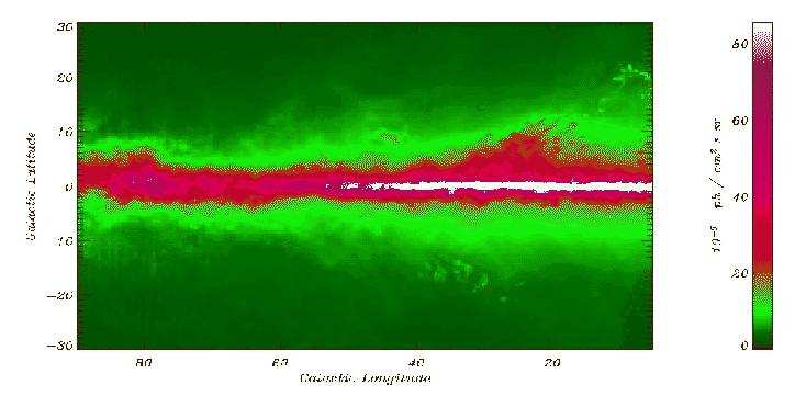$\begin{figure} \centerline{\psfig{figure=fig_model/agile1_cb.eps,width=16cm,height=8cm,angle=0}} \end{figure}$

**Figure 3.2:** Contribution of HI regions to AGILE model, for the first Galactic quadrant. The colorscale is the same shown by the colorbar of figure 3.1.
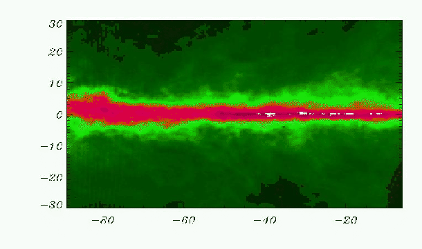$\begin{figure} \centerline{\psfig{figure=fig_model/hi_1.eps,width=13.5cm,height=8cm,angle=0}} \end{figure}$

**Figure 3.3:** Contribution of molecular clouds to AGILE model, for the first Galactic quadrant. The colorscale is the same shown by the colorbar of figure 3.1.
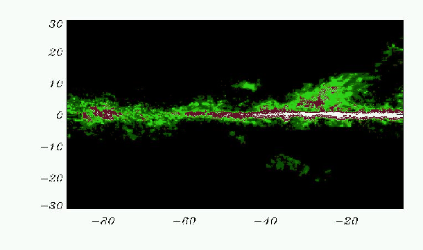$\begin{figure} \centerline{\psfig{figure=fig_model/h2_1.eps,width=13.5cm,height=8cm,angle=0}} \end{figure}$

**Figure 3.4:** Contribution of the interstellar radiation field to AGILE model, for the first Galactic quadrant. The colorscale is the same shown by the colorbar of figure 3.1.
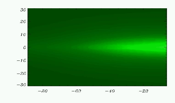$\begin{figure} \centerline{\psfig{figure=fig_model/isrf_1.eps,width=13.5cm,height=8cm,angle=0}} \end{figure}$

**Figure 3.5:** The AGILE emission model for the second Galactic quadrant. The colorscale is the same shown by the colorbar of figure 3.1.
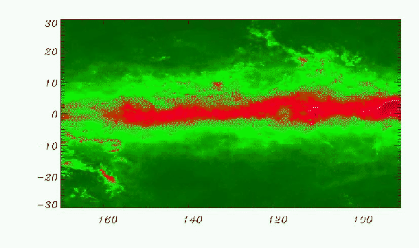$\begin{figure} \centerline{\psfig{figure=fig_model/agile_2.eps,width=13.5cm,height=8cm,angle=0}} \end{figure}$

**Figure 3.6:** Contribution of HI regions to AGILE model, for the second Galactic quadrant. The colorscale is the same shown by the colorbar of figure 3.1.
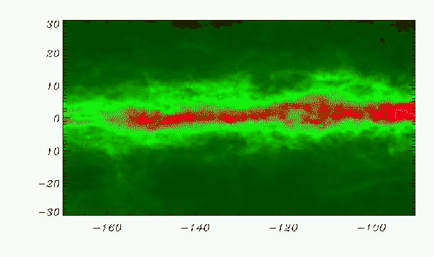$\begin{figure} \centerline{\psfig{figure=fig_model/hi_2.eps,width=13.5cm,height=8cm,angle=0}} \end{figure}$

**Figure 3.7:** Contribution of molecular clouds to AGILE model, for the second Galactic quadrant. The colorscale is the same shown by the colorbar of figure 3.1.
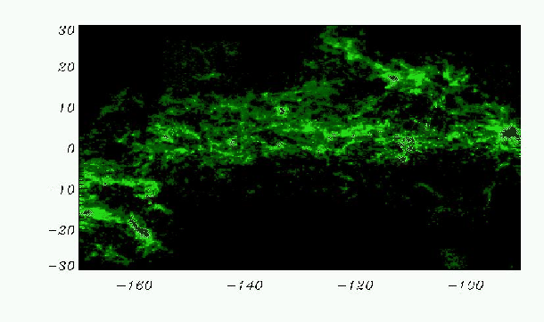$\begin{figure} \centerline{\psfig{figure=fig_model/h2_2.eps,width=13.5cm,height=8cm,angle=0}} \end{figure}$

**Figure 3.8:** Contribution of the interstellar radiation field to AGILE model, for the second Galactic quadrant. The colorscale is the same shown by the colorbar of figure 3.1.
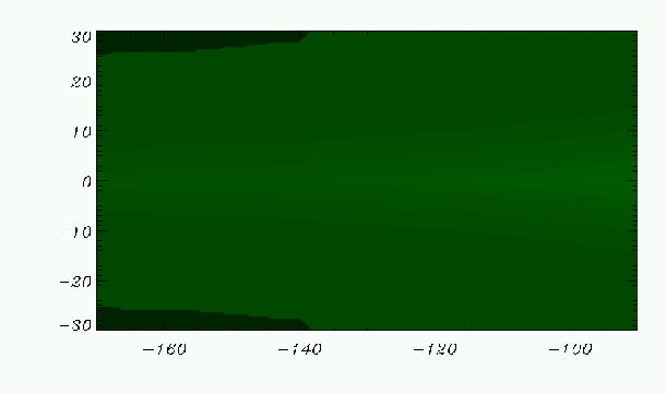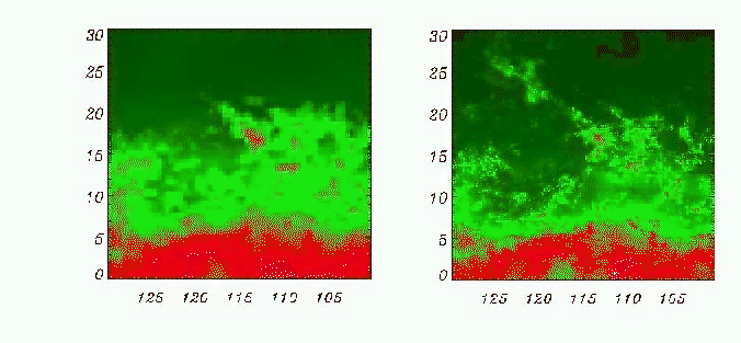
$\begin{figure} \centerline{\psfig{figure=fig_model/isrf_2.eps,width=13.5cm,height=8cm,angle=0}} \end{figure}$

**Figure 3.9:** Comparison between the EGRET (left) and AGILE (right) diffuse emission model for the Polaris Flare regions. The colorscale is the same shown by the colorbar of figure 3.1.
$\begin{figure} \centerline{\psfig{figure=fig_foreground/egretagile_polaris.eps,width=15cm,height=7cm,angle=0}} \end{figure}$

Next: New vs old model Up: Observing the Diffuse Emission Previous: Observing the Diffuse Emission Contents

Andrea Giuliani 2005-01-21