Next: Diffuse matter distribution Up: Modeling the Gamma-Ray Emission Previous: The dynamical ambiguity Contents

Rotation curve

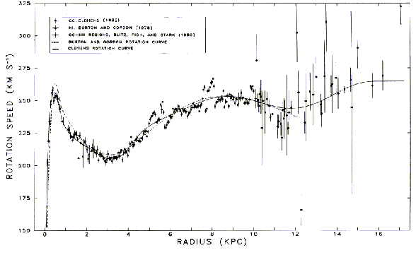
**Figure 2.4:** Plots of the rotation speed versus galactocentric radius. The solid line correspond to the polynomial fit [Clemens, 1985].
$\begin{figure} \centerline{\psfig{figure=fig_model/clemens.eps,height=8cm,width=13cm,angle=0}} \end{figure}$

In order to use the deprojection technique described above it is essential to exactly know the function $\Omega(r)$ . The rotation curve we assume in the model is the one parameterized by [Clemens, 1985], and scaled for a galactic center distance of 8.5 kpc.
This curve was determined for the northern disk component of the Galaxy combining the Massachusetts-Stony Brook Galactic plane CO survey with data for HI in the nuclear region, outer CO - HII regions and globular clusters. The curve, obtained by fitting the data with a polynomial, is shown in figure 2.4.

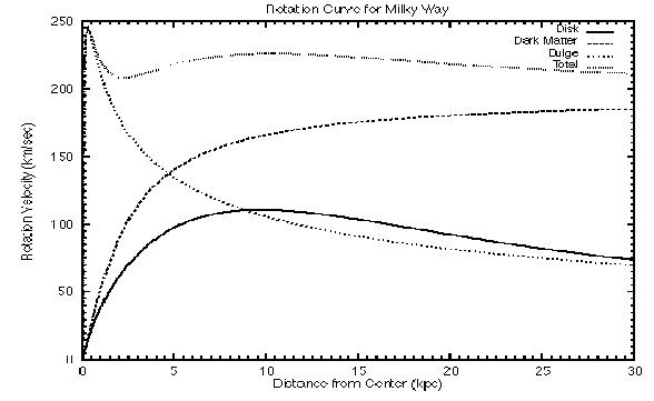
**Figure 2.5:** The observed rotation curve can be decomposed into the individual parts contributed by each component of the Galaxy: the disk (represented by the lowest solid line), the bulge plus the stellar halo (dotted line), and dark matter (dashed line).
$\begin{figure} \centerline{\psfig{figure=fig_model/curve_comp.eps,height=8cm,width=13cm,angle=0}} \end{figure}$

Next: Diffuse matter distribution Up: Modeling the Gamma-Ray Emission Previous: The dynamical ambiguity Contents

Andrea Giuliani 2005-01-21