On-ground tracks reconstruction

The on ground reconstruction processing is based on the same Kalman filter presented in the previous section, nevertheless some refinements have been introduced in order to improve the reconstruction performances. The main refinement consist in the use of Kalman filter to estimate the energy of the single tracks, which, in turn is used as input of the Kalman filter iteratively. Therefore we find that the AGILE Tracker, thanks to its excellent spatial resolution, can by itself provide a good estimate of the incident photon energy from the multiple scattering of $e^+$/$e^-$ passing through the converter planes.

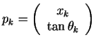
Figure 4.10: Angles definition describing the slopes of the electrons pair.

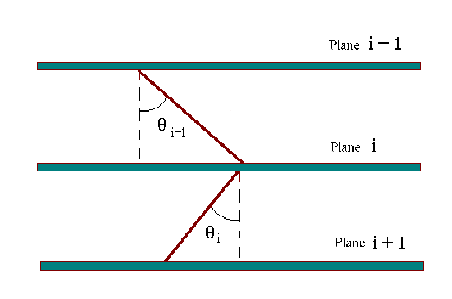In fact it is possible to estimate the energy of the electrons from the aspect of their tracks because when an electron passes through a medium undergoes scattering due to interaction with atomic nuclei of the material; smaller the energy, greater the effect. The angular deviation of electrons due to interaction with the material has approximately a Gaussian distribution. Also the projection of this deviation in a view of the instrument has a Gaussian distribution, with standard deviation:

$$\theta_{rms} = \frac{13.6}{E_{e}[MeV]}\sqrt{\frac{z}{X_{0}}}\left(1+0.038 \ln {\frac{z}{X_{0}}}\right)$$ (4.16)

where z is the thickness and $X_0$ is the radiation length of the material. Therefore, once fixed thickness and material, the average scattering angle depends only on particle energy.

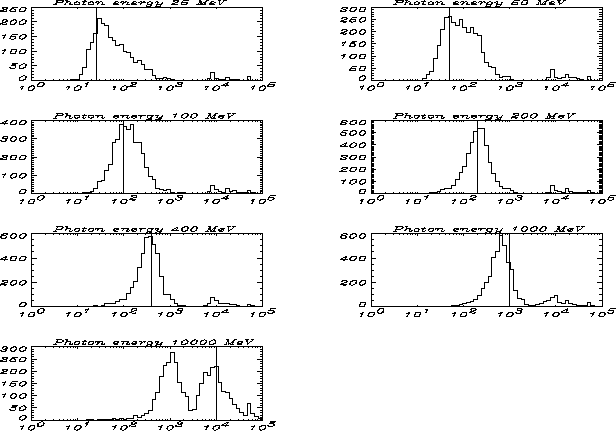
Figure 4.11: Distribution of energy reconstructed with the 'Multiple scattering' method for photons of several energies (photons are 30 degrees off-axis). On the horizontal axis is the reconstructed energy in MeV. The vertical solid line indicates the true energy

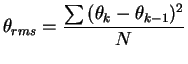
The energy evaluation exploits the fact that for every track the electron slope deviation at every plane can be easily measured. It is therefore possible to estimate the energy inverting the equation (4.16), assuming $\theta_0$ equal to the root mean square of these deviations and assuming:

$$\theta_{rms} = \frac{\sum{(\theta_k - \theta_{k-1})^2}}{N}$$ (4.17)

where $\theta_k$ is the inclination of particle track after the k-th plane and N is the number of crossed planes. This technique is limited by the small number of possible measurements of deviations in one single track (for a track passing through $N_p$ planes N is equal to $N_p - 2$).
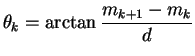
The inclination of a track at the k-th plane ($\theta_k$) can be derived in a simple way :

$$\theta_k = \arctan{\frac{m_{k+1}-m_k}{d}}$$ (4.18)

where $m_k$ is the electron passage coordinate at the k-th plane and d is the distance between two planes. The error on $m_k$ corrupts the measurement of multiple scattering and hence of energy, especially when the scattering angles give deviation comparable or smaller than these errors.
In order to compensate for these errors a Kalman filter can be applied to fit the track. In this way it is possible to obtain a better knowledge of the particle path coordinates and, hence, of $\theta_k$.
The fit obtained by the Kalman filter is a set of vectors $p_k$ with elements:

$$p_{k}=\left(\begin{array}{c} x_k \\ \tan\theta_{k} \\ \end{array} \right)$$ (4.19)

therefore the track inclination at every plane can be immediately derived. The Kalman filter needs an evaluation of the particle energy to calculate the fit of the track, and hence the precision obtainable with this kind of fit depends on precision of energy value. The problem needs to be addressed in an iterative way. An arbitrary energy can be used to start executing the Kalman filter; the values obtained give an evaluation of energy (through eq. 4.17 and 4.16) which is the input for a second Kalman filter. The iteration carries on until the energy values converge.
The distributions of photon energies reconstructed with the method described above are shown in figure 4.11. The simulated photons have the same incoming direction ( $\theta= 30^{\circ} \; \phi=70^{\circ}$) but different energies (from 25 MeV up to 10 GeV).
Table 4.2 shows the three parameters used to describe the distributions. The first parameter, $E_m$, is the geometric mean of values. The ratio $\Delta$E/$E_m$ indicates the width of distribution. Two "68% containment radius" has been calculated for energies both below and above $E_m$ and $\Delta$E represents the sum of two. $\Pi$ is the percentage of events with energy reconstructed in the range $\frac{E_{true}}{1.62} < E < 1.62 E_{true}$ . In this way the range is symmetric with respect to $E_{true}$ (in a logarithmic scale) and the width of range is equal to $E_{true}$. Hence if $\Pi$ equal to $68 \%$, $\Delta$E/$E$ is equal to 1. From the results shown in figure and in table it can be seen that this method gives good results for intermediate energies (100, 200, 400 MeV and partially at 50 MeV). Photons with very low energies (25 MeV) are badly reconstructed due to their complex morphology and this in turn affects their energy measurement. Photons with high energy (1 - 10 GeV) have multiple scattering angles equal or smaller than the tracker intrinsic resolution (about 0.36 degrees), hence the multiple scattering evaluation is affected by measurement errors.

Table 4.2: Parameters of reconstructed energy distributions. All photons are 30 degrees off-axis

Photon energy	$E_m$ [MeV]	$\Delta$E/$E_m$	$\Pi$
25 MeV	69	2.9	37 %
50 MeV	116	2.2	37 %
100 MeV	155	1.8	46 %
200 MeV	259	1.5	56 %
400 MeV	435	1.6	57 %
1 GeV	846	6.4	40 %
10 GeV	3050	4.1	24 %