Spectra extraction
In this example, we will create a wavelength calibration relation ($\lambda \rightarrow$ pix) and we will use it to extract a 2D (LUCI) spectrum lambda calibrated. We will see how to:
- extract a sky 1D spectrum (the background spectrum)
- fit expected line positions with a gaussian model
- fit a polynomial to obtain the wavelength calibration relation
- apply this relation on the raw frame to obtain 2D extracted spectrum
- create the WCS of spectrum from scratch and save it
Keys: astropy models, numpy polynomial, interpolator, wcs
Wavelength calibration relation
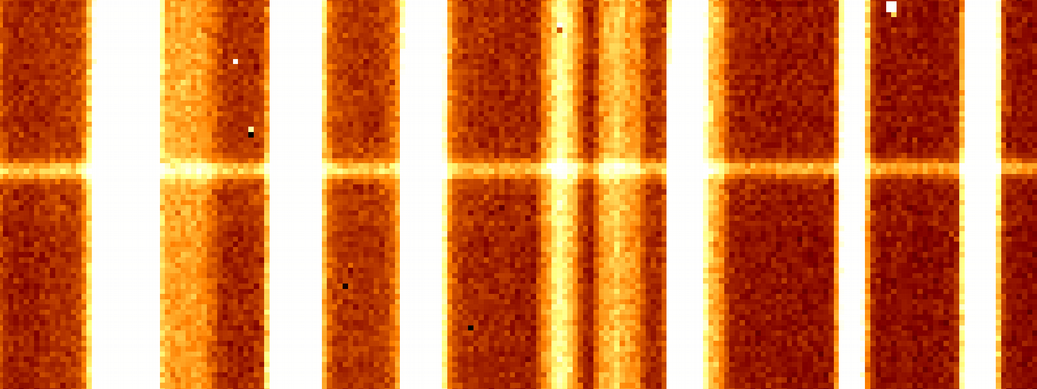
The idea is to use OH lines (near infrared) of raw LUCI frame to derive the relation from Å to pixels, using OH lines (the sky lines) as reference positions.
# Load the frame data
import numpy as np
from astropy.io import fits

with fits.open('data/luci1.20170418.0030.fits.gz') as images:
    data = images[0].data.astype(float) #Convert int16 into floats
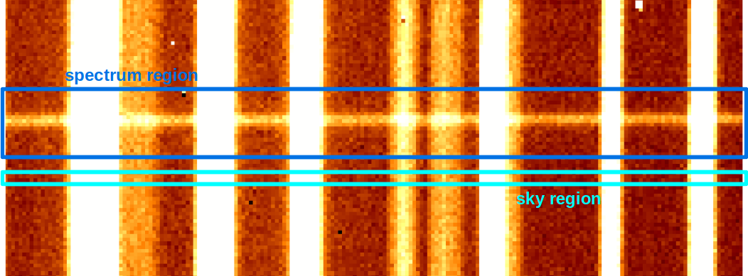
Create a sky spectrum
- We identify a region on the frame near the spectrum to extract, without any other objects (the "sky region" in cyan on the picture).
- Use this region to compute a wavelength calibration model $$p:\lambda \rightarrow pix\hspace{1cm} p(\lambda) = \sum_{i=0}^{n} c_i\lambda^i $$
- Apply the model to the region containing the target (the blue region)
The strong assumption is: no optical distortions exist along the spatial direction, i.e. the variation in $\lambda$ is just along the $x$ direction of the picture (moving along $y$ axis $\lambda$ doesn't change)
The sky spectrum
Create the 1D spectrum
rows=data[1080:1090,:] # Select rows
sky=rows.mean(axis=0) # Create 1D sky spectrum
and display it
#%matplotlib qt
%matplotlib notebook
import matplotlib.pyplot as plt
fig = plt.figure("Sky 1D spectrum")
plt.plot(sky)

Measure line positions
The idea is to find bright and isolated lines (we use Rousselot et al. 2000 as catalog) and compute their positions on the frame (e.g. fitting a gaussian)
#~600pix 16030.83A
flux=sky[560:640]
pix=np.arange(560, 640)

plt.cla()
plt.plot(pix, flux, 'ko', color='gray', alpha=0.5)
plt.plot(pix, flux, '--', color='gray', alpha=0.5)
We can use scipy.otimize.curve_fit like in the previous example or use tools like astropy models
astropy.modelling
astropy.modeling provides a framework for representing models and performing model evaluation and fitting (with parameter constraints) of: 1-D models, 2-D models and compound models
from astropy.modeling import models
model=models.Gaussian1D(mean=600) #Define the model
This module provides also the Fitters: wrappers around some Numpy and Scipy fitting functions. All Fitters can be called as functions
from astropy.modeling import fitting
fitter=fitting.LevMarLSQFitter() # Levenberg-Marquardt algorithm and least squares statistic
Fit the line
gauss=fitter(model, pix, flux) #Compute the fit
In the model instance are stored the fitted parameters, they can be retrieved by name(.param_names)
gauss.param_names
gauss.mean
fitter.fit_info
Errors of the fit on the parameters are stored in the fitter instance (same order of parameters model)
fitter.fit_info['param_cov'] #Covariance matrix on fit parameters
var =  np.diag(fitter.fit_info['param_cov']) # variance on paramters
err = np.sqrt(var)
Display the fit results
#Display the fitted model
xx=np.linspace(560, 640, 1000)
plt.plot(xx, gauss(xx), color='green')
Repeat this recipe
Since we want obtain this measure for a set of lines, we iterate this fitting recipe for a pool of selected lines.
In the example directory there is the wcalib.py script which does that.
This script contains a dictionary with the lines (in Angstrom) and as values, the raw expected positions on the frame (in pixels) as keys. The script loops over the line positions and, for each line, computes a gaussian fit. The results are saved into the tmp/line_positions.dat file.
%pfile ../examples/wcalib.py
%run ../examples/wcalib.py
%cat tmp/line_positions.dat
Display computed positions
#Load the data
positions = np.loadtxt("tmp/line_positions.dat")

plt.cla() #Clear the plot
plt.plot(sky) #Plot the sky
plt.vlines(positions[:,1], 0, sky.max(), color='red') #plot the lines

#Add labels to identify lines
for row in positions:
    plt.text(row[1], 8000, f"$\lambda$ {row[0]}", rotation='vertical', fontsize='x-large')
Compound models
Models can be combined together in a simple way. Here we briefly see, how to combine models, to fit a double gaussian on a pair of lines quite close each other.
#Defined a sub region for fit with 2 sky lines very close
start, stop = 1705, 1750
pix = np.arange(start, stop)
lines = sky[start:stop]

fig = plt.figure()
plt.plot(pix, lines)
plt.plot(pix, lines, 'o', alpha=0.5)

Define and fit the compound model
#Defined the new model
cmodel = models.Gaussian1D(mean=1725, amplitude=700.) + \
        models.Gaussian1D(mean=1735, amplitude=700.) + \
        models.Const1D(amplitude=100)

#Use the previous fitting instance on the new compound model
double_gauss=fitter(cmodel, pix, lines)

#Check the results
xx=np.linspace(pix[0], pix[-1], 1000)
plt.plot(xx, double_gauss(xx), color='magenta')
def tiedf(model):
    return model.mean_0+15.0

cmodel.amplitude_0.fixed=True
cmodel.mean_1.tied = tiedf
tied_gauss=fitter(cmodel, pix, lines)
plt.plot(xx, tied_gauss(xx), color='green')
Find the lambda calibration relation
We have to find the polynomial relation to convert wavelength values (in Angstrom, the expected lines positions) into pixels (the measured line positions in pixels on the frame)
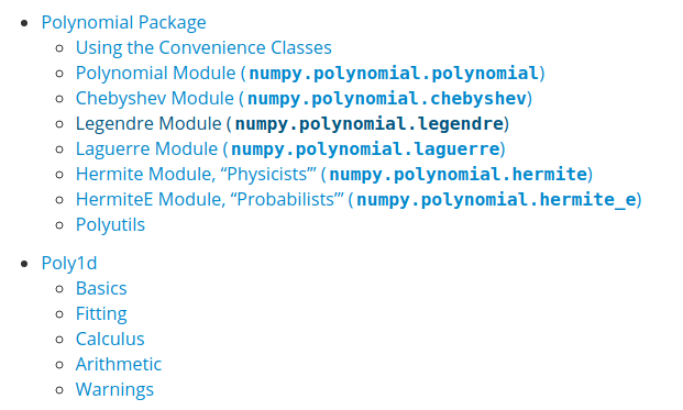
$$ p(\lambda) = \sum_i c_i\lambda^i $$numpy.polynomials
Polynomials in NumPy can be created, manipulated, and even fitted using the classes of the numpy.polynomial package.
The newer Polynomial package is more complete than older numpy.poly1d (prior to Numpy 1.4) and its convenience classes are better behaved in the numpy environment. Therefore Polynomial is recommended for new coding.
NOTE: The various routines in the Polynomial package all deal with series whose coefficients go from degree zero upward, which is the reverse order of the Poly1d convention.
Display the measures
We start displaying points and errors computed, just to have a rough idea about the relation we are looking for.
fig=plt.figure()
plt.errorbar(positions[:,0],positions[:,1],yerr=positions[:,2],fmt='.r')

$$p(\lambda)$$
from numpy.polynomial import polynomial

waves = positions[:, 0]
pixels = positions[:, 1]
errs = positions[:, 2]

c3=polynomial.polyfit(waves, pixels, 3, w=1/errs)
c3
Create the polynomial
# Define the polynomial starting from it's coefficients
p3 = polynomial.Polynomial(c3)
p3
p3.deriv()
Plot polynomial and residuals
#Define lambda range for plot reasons
w = np.linspace(waves[0], waves[-1], 10000)

#New plotting window with 2 subplots
fig=plt.figure()
ax1=fig.add_subplot(121)

#The points
ax1=plt.errorbar(waves, pixels,yerr=errs,fmt='.r', label="positions")

#The polynomial p3(w)=evaluate polynomial in all points of w
ax1=plt.plot(w, p3(w), color='green', label="3rd order")
plt.legend()

#The with residuals
ax2 = fig.add_subplot(122)
ax2.plot(waves, p3(waves)-pixels, 'o', color='orange')

#Add a reference line
ax2.hlines(0, waves[0], waves[-1], ls='--', alpha=0.3)

Extract the spectra
Select the 2D spectrum region, not lambda calibrated and display it
#Select a slice containing the target
spectrum = data[1075:1125]

#Select a log scale to highlight the object
from matplotlib.colors import LogNorm
fig = plt.figure()
ax=fig.add_subplot(111)
ax.imshow(spectrum[:,500:700], cmap='gray', norm=LogNorm())

Apply wavelength calibration
As final step we want to apply the p3 relation row by row independently. We are allow to do that, since in this example we are assuming no variation of the calibration solution along the cross dispersion direction.
The p3 gives a the "float" pixel of each lambda we want to extract.
wrange=np.arange(16000., 17300, 0.8)
pixs=p3(wrange) # The "float" pixels
wrange,pixs
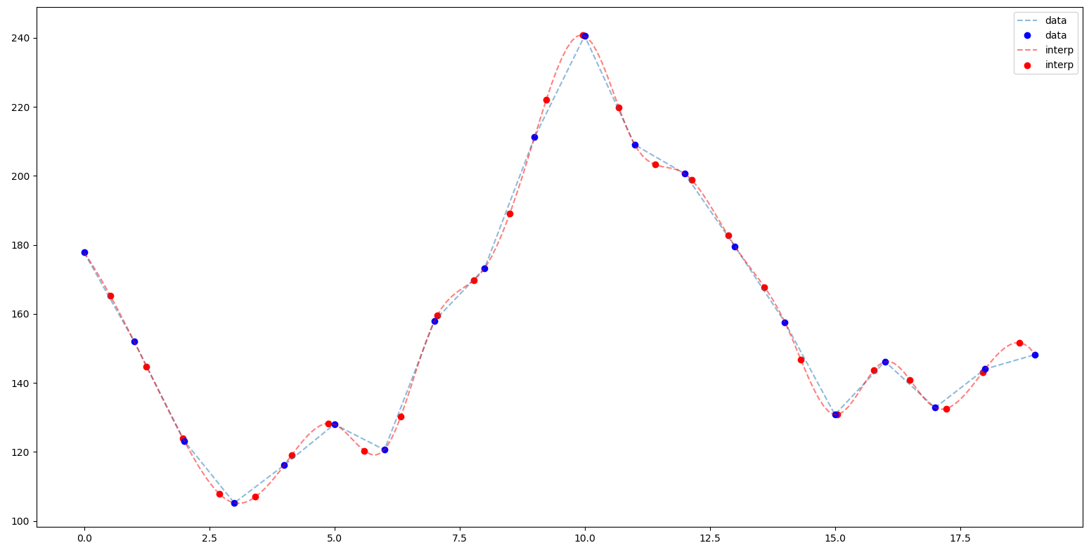
This is a spectrum row details. Red crosses are the point where we want extract the spectrum according with the p3 solution (a subset of pixs array)
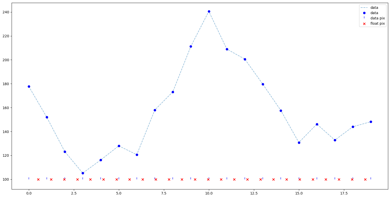 Since we want to have the intensity of the spectrum at these "float" pixels, we must interpolate some how the spectrum in these points
Interpolate the spectrum
There are several general interpolation facilities available in SciPy (Scipy interpolator), for data in 1, 2, and higher dimensions:
a class representing an interpolant (
interp1d) in 1-D, offering several interpolation methods.convenience function griddata offering a simple interface to interpolation in N dimensions (N = 1, 2, 3, 4, …)
functions for 1- and 2-dimensional (smoothed) cubic-spline interpolation, based on the
FORTRANlibrary FITPACK.
from scipy.interpolate import interp1d
interp=interp1d(np.arange(len(spectrum[0])), spectrum, kind='cubic', bounds_error=False)
NOTE: we created the interpolator object with x.shape=(N,) and y.shape=(...,N)
The row detail show before, with the interpolated values
Creating the interpolator in this way: x.shape=(N,) and y.shape=(...,N)) allow us to compute the spectrum 2D interpolated using a single call, without interpolate row by row and loop over rows:
# Less efficient way (and less clear code...) to interpolate the spectrum
spec2d = []
for row in spectrum:
    interp_row=interp1d(np.arange(len(row)), row, kind='cubic', bounds_error=False)
    spec2d.append(interp_row(pixs))
spec2d=interp(pixs)
Create the WCS from scratch
spec2d object is a 2D spectrum wavelength calibrated.
To properly display it, we create a WCS for this spectrum from scratch
from astropy import wcs
from astropy import units as u

w = wcs.WCS(naxis=2)

w.wcs.crpix = [1, 1]

# Along x (dispersion direction) cdelt is the delta lambda increment
# Along y (the cross dispersion direction) no rebinning has been performed cdelt is 1
w.wcs.cdelt = np.array([0.8, 1])

# Starting wavelength along x is 16000A. Starting pixel is 0 (numpy like)
w.wcs.crval = [16000, 0]

w.wcs.cunit =[u.Angstrom, u.pixel]
ax=plt.subplot(projection=w)
ax.imshow(spec2d, cmap='autumn', norm=LogNorm())
specfile = fits.PrimaryHDU(data=spec2d, header=w.to_header())
specfile.writeto("tmp/spectrum.fits", overwrite=True)
2D fit with numpy.polynomial
The polynomial package provides the
polyfit function, just for 1D fitting. For higher dimensional fit numpy doesn't provide a function, but we can use the Pseudo-Vandermonde matrix to perform the fit.
We are going to see how to use it on our usual saddle.dat dataset.
x,y,z=np.loadtxt("data/saddle.dat", unpack=True)

from mpl_toolkits.mplot3d import Axes3D
#Defined a 3D projection figure
fig=plt.figure()
ax = fig.add_subplot(111, projection='3d')

#Plot the data
ax.scatter(x,y,z)

2D poly fit in a nutshell
Given a set of data $x_k,y_k,z_k$ we can rewrite the polynomial relation
$$ z_k = \sum_{i,j} c_{i,j}x_k^iy_k^j\hspace{2cm} (z=ax^2-by^2+c)$$in matrix notation
$$ z = V c \hspace{2cm} z_k=V_kc$$where V is the Pseudo-Vandermonde matrix defined by (here for details)
$$ V_k = [1, y, ..., y^m, x, xy, ..., xy^m, ..., x^n, x^ny, ..., x^ny^m]$$Since we want to find the fit coefficients, we must solve (her for details)
$$ Vc=z \hspace{2cm} V^TVc=V^Tz \hspace{2cm} c=\underbrace{(V^TV)^{-1}V^T}_Hz$$$(V^TV)^{-1}Vz$ in python...
# Pseudo-Vandermonde
V = polynomial.polyvander2d(x, y, (2, 2))

#Compute H
H = np.linalg.inv(V.T@V)@V.T

#Compute the coeffs
coeffs = H@z

#Reshape them according with polyval2d interface
coeffs.shape = (3,3)

#Plot the fitted surface
from matplotlib import cm

X,Y = np.meshgrid(np.linspace(-10,10,20), np.linspace(-10,10,20))

zfit = polynomial.polyval2d(X, Y, coeffs)
surf = ax.plot_surface(X, Y, zfit, cmap=cm.rainbow,
                       linewidth=0, alpha=0.5)