Images
In this exercise we will create a composite (RGB) optical image of a galaxy cluster (from the XXL survey) with the diffuse X-ray emission overplotted as contours. We will see, how to:
- open large images (CFHTLS-Deep field) and extract only an interesting area
- combine images acquired with different filters and create a RGB image
- overplot the contours of the X-ray emission obtained from an X-ray image (XMM-Newton Science Archive)
- overplot markers/patches on selected targets
- save the final image (png, pdf, svg, ...)
Keys: WCS, SkyCoord, Cutout2D, data visualization (images normalization, countour plots, marker, ...), GRB combination, reprojection, Multidimensional image
Open image
from astropy.io import fits

hdulist = fits.open('data/CFHTLS_D-25_g_022559-042940_T0004.fits')
image=hdulist[0]

#image is very large
image.data.shape
WCS
astropy.wcs contains utilities for managing World Coordinate System transformations in FITS files. These transformations map the pixel locations in an image to their real-world units, such as their position on the sky sphere. These transformations can work both forward (from pixel to sky) and backward (from sky to pixel).
It performs three separate classes of WCS transformations:
Core WCS, as defined in the FITS WCS standard, based on Mark Calabretta’s
wcslibSimple Imaging Polynomial (
SIP) convention.table lookup distortions as defined in the FITS WCS distortion
paper.
Each of these transformations can be used independently or together.
#Create the WCS object
from astropy.wcs import WCS
wcs = WCS(image)
wcs
image
Uses
WCSto convert pixels into sky coordinatesNOTE: 0 is the origin parameter (Numpy-like)
coords = wcs.wcs_pix2world(((5090,5115),(5091,5115),(5090,5116)),0, ra_dec_order=True)
coords
- and viceversa
wcs.wcs_world2pix(coords,0)
Cutout2D: extract a subimage
The Cutout2D class can be used to create a postage stamp of an image (2D array). If an optional WCS object is input to Cutout2D, then the Cutout2D object will contain an updated WCS corresponding to the cutout array.
In this example, we will work with the WCS. The same arrangement can be performed in using pixels.
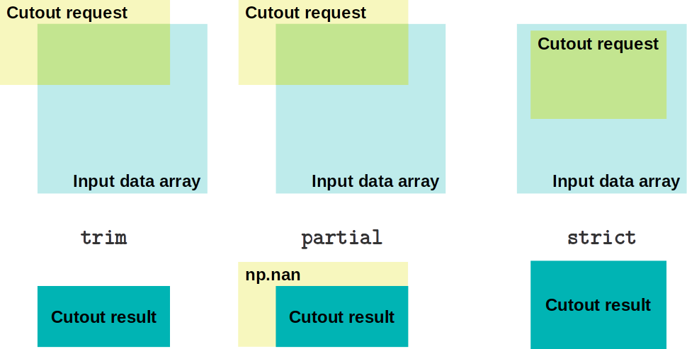
There are three modes for creating cutout arrays:
trim(default): partial overlap of the cutout array and the input data array is sufficient. The result can be smaller than the requested sizepartial: partial overlap of the cutout array and the input data array is sufficient. The cutout will never be trimmed, it will be filled with fill_value (defaultnumpy.nan)strict: will raise an exception if the cutout is not fully contained
#Define the center
from astropy.coordinates import SkyCoord
center = SkyCoord('2h25m31s -4d14m27.78s')

#Create the thumbnail
from astropy import units as u
from astropy.nddata import Cutout2D
thumb=Cutout2D(image.data, center, (4*u.arcmin, 3*u.arcmin),wcs=wcs)
Cutout2D?
SkyCoord and angles
The coordinates package provides classes for representing a variety of celestial/spatial coordinates and their velocity components, as well as tools for converting between common coordinate systems in a uniform way.
c = SkyCoord('2:25:31 -4:14:27.78', unit=(u.hourangle, u.deg), frame='icrs')
center, c
- coordinates transformations
c.galactic, c.fk4, c.fk5
- retrieve angles from coordinates
c.ra, c.dec
- angle conversions
c.ra.hour, c.ra.arcmin, c.ra.rad, c.ra.deg
The distance
SkyCoord has the additional distance attribute
c2 = SkyCoord('2:25:31 -4:14:27.78', unit=(u.hourangle, u.deg), distance=574*u.kpc)
c3 = SkyCoord('1:02:31 -2:10:27.78', unit=(u.hourangle, u.deg), distance=123*u.kpc)
c3
- compute distances
c2.separation(c3), c2.separation_3d(c3)
- quick way to get coordinates for named objects (
Sesame)
SkyCoord.from_name('NGC 1142')
Save the thumbnail
#Create a new fits image
data = thumb.data
header = thumb.wcs.to_header()
primary = fits.PrimaryHDU(data=data, header=header)
primary.writeto("tmp/g.fits", overwrite=True)
thumb.wcs.to_header()
# Preserve the orignal header and update the WCS
original_header = image.header
original_header.update(thumb.wcs.to_header())
primary = fits.PrimaryHDU(data=data, header=original_header)
primary.writeto("tmp/g.fits", overwrite=True)
Now we extract one subimage for each filter and save it
#Loop over filters
for _filter in ('g', 'r', 'i'):
    #Open image creating the the proper file name
    hdulist = fits.open('data/CFHTLS_D-25_%s_022559-042940_T0004.fits' % _filter)

    #Get the image a wcs
    image=hdulist[0]
    wcs = WCS(image)

    #Extract subimage
    thumb=Cutout2D(image.data, center, (4*u.arcmin, 3*u.arcmin),wcs=wcs)

    #Save on disk
    primary = fits.PrimaryHDU(data=thumb.data, header=thumb.wcs.to_header())
    primary.writeto(f"tmp/{_filter}.fits", overwrite=True) #Different str syntax
    hdulist.close()
label="alpha"
value=2.12345E-7
"%s=%.3e" % (label, 5*value) # Old style
f"{label}={5*value}"
f"{label}={5*value:.3e}"
Data visualization
astropy.visualization provides functionality that can be helpful when visualizing data. This includes
- a framework for plotting Astronomical images with coordinates with Matplotlib
- functionality related to image normalization (including both scaling and stretching)
- smart histogram plotting
- RGB color image creation from separate images
#Open new data and wcs
with fits.open("tmp/g.fits") as hdulist:
    g = hdulist[0].data.copy()
    wcs = WCS(hdulist[0]) #All 3 images have the same WCS in this example
with fits.open("tmp/r.fits") as hdulist:
    r = hdulist[0].data.copy()
with fits.open("tmp/i.fits") as hdulist:
    i = hdulist[0].data.copy()
#%matplotlib qt
%matplotlib notebook
from matplotlib import pyplot as plt

fig=plt.figure("Display images")
ax11=fig.add_subplot(221, projection=wcs)
ax11.imshow(g)
ax11.grid(color='white', ls='--', alpha=0.5)
ax11.set_xlabel('RA')
ax11.set_ylabel('Declination')

ax21=fig.add_subplot(223)
ax21.set_yscale('log')
_ = ax21.hist(g.ravel(), bins=100)
A simple way to "see" an image is to exclude the extreme values (e.g. using a sigma clipping)
from astropy.stats.sigma_clipping import sigma_clip

clipped_g = sigma_clip(g, sigma=5, maxiters=3)
ax12=fig.add_subplot(222, projection=wcs)
ax12.imshow(g, vmin=clipped_g.min(), vmax=clipped_g.max())
ax12.grid(color='white', ls='--', alpha=0.5)
ax12.set_xlabel('RA')
ax12.set_ylabel('Declination')

ax22=fig.add_subplot(224)
_ = ax22.hist(clipped_g.ravel(), bins=300)
Image stretching and normalization
Now, we will see how to modify an image (arrays), for a better visualization. Two main types of transformations are provided:
- Normalization (Interval objects) to the $\left[0,1\right]$ range using lower and upper limits where $x$ represents the values in the original image and $y$ the transformed image:
In addition, classes are provided in order to identify lower and upper limits for a dataset based on specific algorithms.
- Stretching (Stretch objects) of values in the $\left[0,1\right]$ range to the $\left[0,1\right]$ range using a linear or non-linear function:
Intervals
Several classes are provided for determining intervals and for normalizing values in this interval to the $\left[0,1\right]$ range:
The zscale example
We use zscale interval class to find image limits
from astropy.visualization import ZScaleInterval

fig=plt.figure("zscale")
ax1=fig.add_subplot(121, projection=wcs)

zscale=ZScaleInterval()
vmin,vmax=zscale.get_limits(g)

im1=ax1.imshow(g, vmin=vmin, vmax=vmax)
fig.colorbar(im1)

We can use z-scale (DS9 like) to rescale the image
ax2=fig.add_subplot(122, projection=wcs,  sharex=ax1, sharey=ax1)
im2=ax2.imshow(zscale(g))
fig.colorbar(im2)
fig=plt.figure()

#Defined the scale
zscale=ZScaleInterval()
gmin, gmax = zscale.get_limits(g)
rmin, rmax = zscale.get_limits(r)
imin, imax = zscale.get_limits(i)

ax11=fig.add_subplot(231)
ax11.imshow(g, vmin=gmin, vmax=imax, cmap="Blues", origin='lower') #lower parameter!

ax12=fig.add_subplot(232)
ax12.imshow(r, vmin=rmin, vmax=rmax, cmap="Greens", origin='lower')

ax13=fig.add_subplot(233)
ax13.imshow(i, vmin=imin, vmax=imax, cmap="Reds", origin='lower')

hrange=[min(gmin, rmin, imin), max(gmax, rmax, imax)]

#Plot histograms
ax21=fig.add_subplot(234)
_ = ax21.hist(g.ravel(), range=hrange, bins=100, color='blue')
ax22=fig.add_subplot(235)
_ = ax22.hist(r.ravel(), range=hrange, bins=100, color='green')
ax23=fig.add_subplot(236)
_ = ax23.hist(i.ravel(), range=hrange, bins=100, color='red')

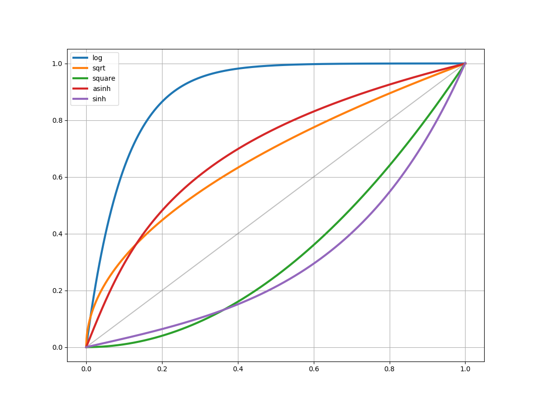
Stretch
In addition to classes that can scale values to the $\left[0:1\right]$ range, a number of classes are provided to stretch the values using different functions. These map a $\left[0:1\right]$ range onto a transformed $\left[0:1\right]$ range.
AsinhStretchBaseStretchContrastBiasStretchHistEqStretchLinearStretchLogStretchPowerDistStretchPowerStretchSinhStretchSqrtStretch-
NOTE: The stretch functions are similar but not always strictly identical to those used in e.g. DS9.
Matplotlib normalization
Matplotlib provides a custom normalization and stretch when displaying data by passing a matplotlib.colors.Normalize object
NOTE: Stretches can also be combined with other stretches, just like transformations. The resulting CompositeStretch can be used to normalize Matplotlib images like any other stretch.
from astropy.visualization import *

fig=plt.figure("Image normalize")

# Create an ImageNormalize object
norm = ImageNormalize(image, interval=ManualInterval(0.2, 5.0),
                      stretch=AsinhStretch()+PowerDistStretch(3.0))
im = plt.imshow(g, norm=norm, origin='lower')

Parameters in stretch functions
Some stretching functions, require input parameter used to tune the stretch. For example the alternative power stretch
$$ y = \frac{a^x-1}{a-1}$$Automatic creation of RGB image
Lupton et al. (2004) describe an “optimal” algorithm for producing red-green-blue composite images from three separate high-dynamic range arrays. This method is implemented in make_lupton_rgb as a convenience wrapper function
# Input: red, green and blue
rgb_lupton = make_lupton_rgb(i, r, g)
rgb_lupton
RGB manual combination
We want to combine together 3 filters to obtain a RGB image
new_images=[]
#Loop over images: g, r, i
for image in (i, r, g):
    #Simple example: use a custom recipe
    median = np.median(image.data)
    delta = (image.max()-median)/200.
    high = median + delta
    low = median - delta/8.

    #Define transformation
    T = ManualInterval(low, high)

    #Apply transformation and create a new image
    new_images.append(T(image))

grb_manual = np.dstack(new_images)
Display the RGB images
fig=plt.figure()

#Plot histograms
axm=fig.add_subplot(121, projection=wcs)
axm.set_title("Manual")
axm.imshow(grb_manual, origin='lower')
axm.grid(color='white', ls='--', alpha=0.5)
axm.set_xlabel("RA")
axm.set_ylabel("Declination")

axl=fig.add_subplot(122, projection=wcs, sharex=axm, sharey=axm)
axl.set_title("Lupton")
axl.imshow(rgb_lupton, origin='lower')
axl.grid(color='white', ls='--', alpha=0.5)
axl.set_xlabel("RA")
axl.set_ylabel("Declination")

Overplot contours
Open the image selected to show contour levels, in this case an X-ray image from XMM, and select the region of interest as previously done in creating the RGB image
with fits.open("data/MLS2_xmm_img.fits.gz") as hdulist:
    xmm = hdulist[0].copy()

x = Cutout2D(xmm.data, center, (4*u.arcmin, 3*u.arcmin),wcs=WCS(xmm))
x.shape
g.shape
NOTE: In this case the image has not the same WCS as the CFHT images. We need to reproject the image onto the WCS of the GRB image
from reproject import reproject_interp
array, footprint = reproject_interp((x.data, x.wcs), wcs, shape_out=g.shape)
array.shape
We want to use the X-ray image to compute the contour plot of the X-ray emission and oveplot it onto the RGB image
axm.contour(array, levels=(2.5, 5, 7.5, 10, 12.5), colors='pink')
axm
To plot smoother contours, use the scipy.ndimage package to smooth the original image and recompute contour on it
import scipy.ndimage as ndimage
sarray = ndimage.gaussian_filter(array, sigma=5.0)
axl.contour(sarray, levels=(2.5, 5, 7.5, 10, 12.5), colors='cyan')
scipy.ndimage
The scipy.ndimage package provides a number of general image processing and analysis functions that are designed to operate with arrays of arbitrary dimensionality. The package currently includes:
- Filter functions
- Correlation and convolution
- Smoothing filters
- Filters based on order statistics
- Derivatives
- Generic filter functions
- Fourier domain filters
- Interpolation functions
- Spline pre-filters
- Interpolation functions
- Morphology
- Binary morphology
- Grey-scale morphology
- Distance transforms
from astropy.table import Table

catalog=Table.read('data/D1_MLS2_zspec.tbl', format='ascii')
catalog
Marker
Add markes on manual RGB figure
# Retreive marker in pixels
markers=np.array([catalog['ra'], catalog['dec']])

# COnvert pixels in coordinate system positions
pix_markers = wcs.wcs_world2pix(markers.T, 0)

axm.scatter(pix_markers[:,0], pix_markers[:,1], s=30, edgecolor='red', facecolor='none')
markers=np.array([catalog['ra'], catalog['dec']])
markers.T
Patch
Add patches to the Lupton RGB figure
from matplotlib.patches import RegularPolygon

for ra,dec in catalog['ra', 'dec']:
    c = RegularPolygon((ra, dec), 5, 0.001, edgecolor='yellow', facecolor='none',
              transform=axl.get_transform('fk5'))
    axl.add_patch(c)
Save the figure
#Prepare the canvas
fig=plt.figure(figsize=[4.0, 4.0], dpi=300)

ax=plt.subplot(projection=wcs)
ax.imshow(grb_manual, origin='lower')
ax.grid(color='white', ls='--')
ax.set_xlabel("RA", fontsize='x-small')
ax.set_ylabel("Declination", fontsize='x-small')
ax.tick_params(labelsize='xx-small')
#Display patches
for ra,dec in catalog['ra', 'dec']:
    c = RegularPolygon((ra, dec), 5, 0.001, edgecolor='yellow', facecolor='none',
              transform=ax.get_transform('fk5'))
    ax.add_patch(c)

#Display contour
ax.contour(sarray, levels=(2.5, 5, 7.5, 10, 12.5), colors='cyan')

#Select a region
ax.set_xlim(200,800)
ax.set_ylim(400,1000)

#Save
plt.savefig('tmp/cluster.png')
plt.savefig('tmp/cluster.pdf')

!ristretto tmp/cluster.png