$\gamma$-ray spectra visualization and fit
In this example we want fit a power law function on one high energy $\gamma$-ray spectrum (Aharonian et al 2006) acquired by HESS. We will see, how to:
- visualize the spectrum
- overlay on spectrum the model already computed
- fit a new model
- compute the integrated energy of the 2 models
Key: error plot, scatter plot, curve fit, integration
Explore the file
from astropy.io import fits

tev = fits.open('data/TeVJ1826-148.fits')
tev.info()
Open the proper extension (HESS_INFC) and retrieve just data
infc=tev['HESS_INFC'].data
infc
prepare the plot
#%matplotlib qt
%matplotlib notebook
from matplotlib import pyplot as plt

fig = plt.figure("HESS Spectrum")
ax = fig.subplots()

Error bars
Display points and errors
ax.errorbar(infc['ENERGY'], infc['FLUX'], yerr=[infc['FLUX_ERROR_MIN'], infc['FLUX_ERROR_MAX']],
            label='HESS INFC', color='red', fmt='o')
infc
Plot setup
Setup the plot: scales, axes labels and legend
ax.set_xscale("log")
ax.set_yscale("log")
ax.set_xlabel("E(TeV)")
ax.set_ylabel(r"Flux ($\frac{ph}{cm^2sTev}$)") #raw string, no characters escaping
In the same way we can retrieve data model, and plot it as a solid line without error
#Load the model
model=tev['MODEL_HESS_INFC'].data
ax.plot(model['ENERGY'], model['FLUX'], label='model', color='gray')
ax.legend()
model=tev['MODEL_HESS_INFC'].data
model.dtype
from scipy.optimize import curve_fit
optimize.curve_fit
curve_fit requires the definition of our function.
Signature of this function MUST be ydata = f(xdata, *params)
In our case we decide to fit a power law like that
$$N x^{-\alpha} e^{-\frac{x}{x_{off}}}$$The parameters of the function are: $N$, $\alpha$ and $x_{off}$
import numpy as np

def powerlaw(x, N, alpha, x_off):
    return N * np.power(x, -alpha) * np.exp(-x/x_off)
- use the function with scalar
powerlaw(1, 3.0, 2.0, 0.5)
powerlaw(1, 3.0, 2.0, 0.5)
- and with numpy.array objects
_x=np.array([0.5, 1.0, 2.0])
powerlaw(_x, 3.0, 2.0, 0.5)
_x=np.array([0.5, 1.0, 2.0])
powerlaw(_x, 3.0, 2.0, 0.5)
Compute the fit
xdata = infc['ENERGY']
ydata = infc['FLUX']
yerr = infc['FLUX_ERROR_MAX']
popt, pcov=curve_fit(powerlaw, xdata, ydata, sigma=yerr, p0=(1.0, 1, 6.0))
popt, pcov
curve_fit?
Compute the $\chi^{2}$
$$ \chi^2 = \sum_j^n \left( \frac{f(x_j) - y_j}{y_{err}} \right)^2 $$$$ \chi^2_{r} = \frac{\chi^2}{n-n_{p}} $$import numpy as np
chisq = np.sum(((powerlaw(xdata, *popt) - ydata)/yerr)**2)
reduced_chisq = (chisq)/(len(xdata)-len(popt))
powerlaw(xdata, *popt)
Plot the final model
# Compute the fitted function on the grid of x
x=np.linspace(xdata[0], xdata[-1], 1000)
yfit=powerlaw(x, *popt)

#Setup a new figure
fig=plt.figure()
ax = fig.subplots()

#Plot the fitted function
ax.plot(x, yfit, color='blue', label='powerlaw fit')

#Plot data
ax.errorbar(xdata, ydata, yerr=[infc['FLUX_ERROR_MIN'], infc['FLUX_ERROR_MAX']], label='HESS', color='red', fmt='o')

#Plot original model
ax.plot(model['ENERGY'], model['FLUX'], label='model', color='gray', ls='--')
ax.legend()
ax.set_xscale('log')
ax.set_yscale('log')

Fix some parameters
curve_fit assumes $f$ must have this signature ydata = f(xdata, *params) there are not additional options for fixed parameters.
curve_fit provides also the bounds parameter to set a lower and upper limits in parameters space exploration. In any case each lower bound must be strictly less than each upper bound.
# This call raises an error!
popt, pcov=curve_fit(powerlaw, xdata, ydata, sigma=yerr, p0=(2.97, 1, 6.0), bounds=((2.97, 0, 0),
                                                                                    (2.97, 10., np.inf)))
Goal: we must find a way provide some parameter to the final function (the powerlaw in this case), but this parameter can not be a function argument.
We can define an auxiliary function and take advantage of variables scopes.
Variables scope
Variables can only reach the area in which they are defined, which is called scope. Think of it as the area of code where variables can be used. Python supports global variables (usable in the entire program) and local variables.
By default, all variables declared in a function are local variables. To access a global variable inside a function, it’s required to explicitly define global variable.
def powerlaw(x, N, alpha, x_off):
    return N * np.power(x, -alpha) * np.exp(-x/x_off)
We can define "new" powerlaw function, with only 2 free parameter: $\alpha$ and $x_{off}$.
The N parameter is defined out of powerlaw function.
    def powerlaw(x, alpha, x_off):
        return N * np.power(x, -alpha) * np.exp(-x/x_off)
We nest powerlaw inside another function which provides N. In this way N is defined outside powerlaw, but it is in the powerlaw scope.
def powerlawN(N):
    # Variable N lives in this scope
    def powerlaw(x, alpha, x_off):
        return N * np.power(x, -alpha) * np.exp(-x/x_off)
    return powerlaw
powerlawN(2.97e-12) returns a powerlaw with a fixed N, and we can call the curve_fit in this way
popt2, pcov2=curve_fit(powerlawN(2.97e-12), xdata, ydata, sigma=yerr, p0=(1, 6.0))
popt2,pcov2
Comute the integrate energy: scipy.integrate
The scipy.integrate sub-package provides several integration techniques:
- Methods for Integrating Functions given function object
- Methods for Integrating Functions given fixed samples
- Interface to numerical integrators of ODE systems
We use quad function, which use a technique from the Fortran library QUADPACK, on the analytic model
from scipy.integrate import quad

value, err = quad(powerlaw, 0.2, 20, args=tuple(popt))
value
And the simps function, which use the composite Simpson’s rule, to integrate the sampled model.
from scipy.integrate import simps

idx = (model['ENERGY'] >=0.2) & (model['ENERGY'] <=20.0)
value = simps(model['FLUX'][idx], model['ENERGY'][idx])
value
idx
Fill area in plot
xfill = np.linspace(0.2, 20, 100)
ax.fill_between(xfill, 0, powerlaw(xfill, *popt), color='orange')
ax
and close the file
tev.close()
def sum(*args):
    s=0
    for i in args:
        s+=i
    print(s)
sum(1, 2, 3)
sum([1, 2, 3]) # Error!
sum(*[1, 2, 3])
def show(**kargs):
    print(kargs)
    print("keys", *kargs)
show(a=1, b="x")
curve_fit: N dimensional fit
In this example we fit the hyperbolic paraboloid defined by 3 parameters (a, b, c):
$$ z = ax^2-by^2+c $$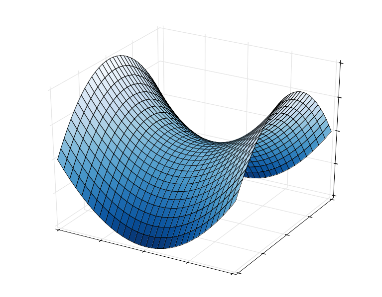
By Nicoguaro - Own work, CC BY 3.0, https://commons.wikimedia.org/w/index.php?curid=20570051
load the observed point
x,y,z=np.loadtxt("data/saddle.dat", unpack=True)
Plot the points in 3D plot
from mpl_toolkits.mplot3d import Axes3D
#Defined a 3D projection figure
fig=plt.figure()
ax = fig.add_subplot(111, projection='3d')

#Plot the data
ax.scatter(x,y,z)

Define the hyperbolic paraboloid function
def hypar(x, y, a, b, c):
  return a*x*x - b*y*y + c
PROBLEM: we can not use hypar function with curve_fit
$f$ interface must be ydata = f(xdata, *params)
popt, pcov = curve_fit(hypar, x, y , z) # x and y not allow!
Define a new interface, where $x$ and $y$ data are packed together into a generic data
def hypar_interface(data, a, b, c):
  _x = data[:len(data)//2]
  _y = data[len(data)//2:]
  return hypar(_x, _y, a, b, c)
prepare the input data for hypar_interface
#Concatenate x,y for curve_fit
input_data = np.concatenate((x, y))
compute the fit
#The invalid syntax just for comparison
popt, pcov = curve_fit(hypar, x, y , z)
#Compute the fit
popt, pcov = curve_fit(hypar_interface, input_data, z)
popt, pcov
Show the results
Evaluate the function on a regular grid of X and Y. Plot the surface obtained by the fit
#Evaluate the function on a grid of values
X,Y = np.meshgrid(np.linspace(-10,10,20), np.linspace(-10,10,20))

zfit = hypar(X, Y, *popt)

#Plot the surface
from matplotlib import cm
surf = ax.plot_surface(X, Y, zfit, cmap=cm.rainbow,
                       linewidth=0, alpha=0.5)