Image data (Numpy array)
In this exercise, we will:
- have a NumPy array overview
- apply array slicing and reduction methods to remove bias from one optical CCD MODS1R frame, computing the bias levels of prescan/overscan regions
Keys: NumPy, array indexing, slicing, view and reduction, astropy.stats and masked arrays
Image Data
#Open the file
from astropy.io import fits

with fits.open('data/mods1r.20171125.0026.fits') as hdulist:
    #Retrieve image data copy
    data = hdulist[0].data.copy()
data
Numpy array
np.arrayis a grid of values- which is indexed by a tuple of integers
- the indexing order is the C language order by default (row major, items go from 1st row left to right, then 2nd row and so on)
- the number of dimensions is the rank of the array
- the
shapeof an array is a tuple of integers giving the size of the array along each dimension - shape can be easily modified
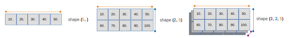
import numpy as np

# 1 dimensional array
a = np.array([10., 20., 30., 40., 50.])

# 2 dimensional array
b = np.array([[ 10., 20., 30., 40.,  50.], \
              [ 60., 70., 80., 90., 100.]])

# 3 dimensional array
c = np.array([[[ 10.,  20.,  30.,  40.,  50.], \
               [ 60.,  70.,  80.,  90., 100.]],\

              [[ 110., 120., 130., 140., 150.], \
               [ 160., 170., 180., 190., 200.]],\

              [[ 210., 220., 230., 240., 250.], \
               [ 260., 270., 280., 290., 300.]]])

# and so on......
Array reshaping
- reshape to obtain new array
#1D array
a_shape = np.arange(0, 15)

#Create 2D array by reshape
b_shape = a_shape.reshape((3, 5))
BE CAREFUL: (we will see later) this is not a new array, but a view of the the original array
b_shape
We can also reshape in place
a_shape.shape=(5,3)
a_shape
Array creation
There are several general mechanisms for creating arrays
import numpy as np
#Array full of 1.0 of length 2
np.ones((2,))
#Empty array of length 4
np.empty((4,))
#Array full of -infinite of length
np.full((5,), -np.inf)
z=np.zeros((3,))
#Array with the same shape of z full of 3.14
np.full_like(z, 3.14)
#Values are generated between the half-open interval [-2.3,1.5) 0.4 is the step
np.arange(-2.3, 1.5, 0.4)
#Returns 5 evenly spaced numbers over the closed interval [-2.3, 1.5]
np.linspace(-2.3, 1.5, 5)
np.linspace(-2.3, 1.5, 5)
import numpy as np
a = np.array([-1, 0, 3])
Numpy array types
- numpy arrays comprise elements of a single data type
- the data type object is accessible through the
.dtypeattribute
# Data type
data.dtype.type  ### All items have the same type: np.array are homogenus!
# Data type name
data.dtype.name
#Memory size (byte) of each elements
data.dtype.itemsize
a
- array dtypes are usually automatically inferred
#a = np.array([-1, 0, 3])
b = np.array([-1.,0.,3.])
a.dtype, b.dtype
- array dtype can be defined by the user
c=np.array(a, dtype=bool)
c
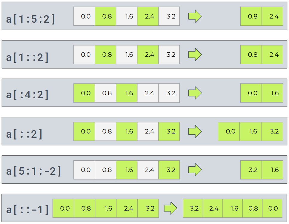
Indexing
- indexes start from 0
a = 0.8*np.arange(0, 5) #Define the array
a[0] # First element
a[4] # Last element
a[4]
- negative indexes are allowed (from right to left)
a[-1] # Last element
a[-5] # First element
a[-5]
- slices are allowed (open right intervals)
#Get 2nd and 3th element [1,3)
a[1:3]
a[1:3]
Basic Slicing
Basic slicing extends Python’s basic concept of slicing to N dimensions. Basic slicing occurs when obj is a slice object (constructed by start:stop:step notation inside of brackets)
Slicing and view
- simple assignments do not create copies of an array (same as Python)
b=a
b is a # True
- slicing operations do not create copies either: they return views of the original array
- an array view contains a pointer to the original data
c = a[3:5]
c+=1
a #changed
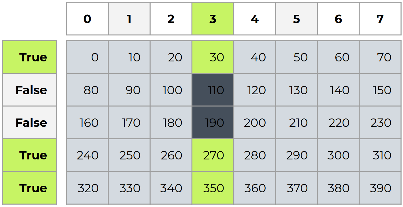
N-d array
Just define the array for examples
a=10.*np.arange(0, 40).reshape((5,8))
a
- retrieve a single element:
row,colindexing
a[0][1] #Element of 1st row, 2nd column
a[0,1] #The same
NOTE: arrays are used to map image data, but arrays indexing is different from image (x,y) coordinates
a[0][1]
Retrieve rows
a[0] #The 1st row
a[0,:]
a[0]
Retrieve matrices
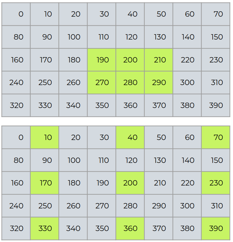
a[2:4,3:6]
a[::2,0::3]
Advanced indexing
There are two types of advanced indexing: integer and boolean. Advanced indexing always returns a copy of the data (contrast with basic slicing that returns a view).
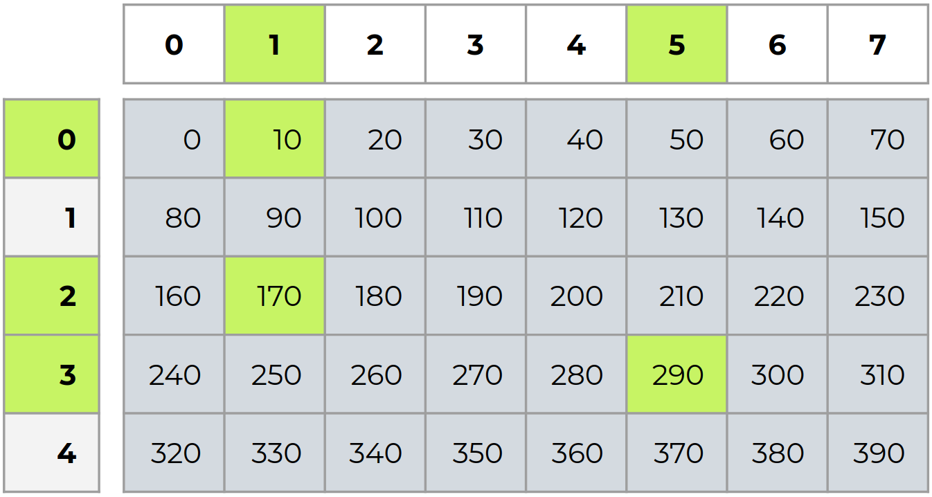
i = np.array([0, 2, 3])
j = np.array([1, 1, 5])
b = a[i,j]
b
i = np.array([True, False, False, True, True])
c = a[:,3][i] # b is not a view of a
c
Scalar operations
a=np.arange(1, 5)
- sum/subtraction
a-0.5 - multiplication
a*2.5 - division
a/2(returns float) - floor division
a//2(rounded away from +infinity) - mod operation
a%3 - power
a**2 - numpy functions
np.log(a)
-5//2.
Arrays operations
a=np.array([1., 2., 3.])
b=np.array([2., -1., 0.])
- sum/subtraction
a-b - multiplication
a*b - float division
a/b - floor division
a//b - mod operation
a%b - power
a**2 - dot product
a.dot(b)ora@b - tensor product
np.tensordot(a,b,axes=0)
np.tensordot(a,b,axes=0)
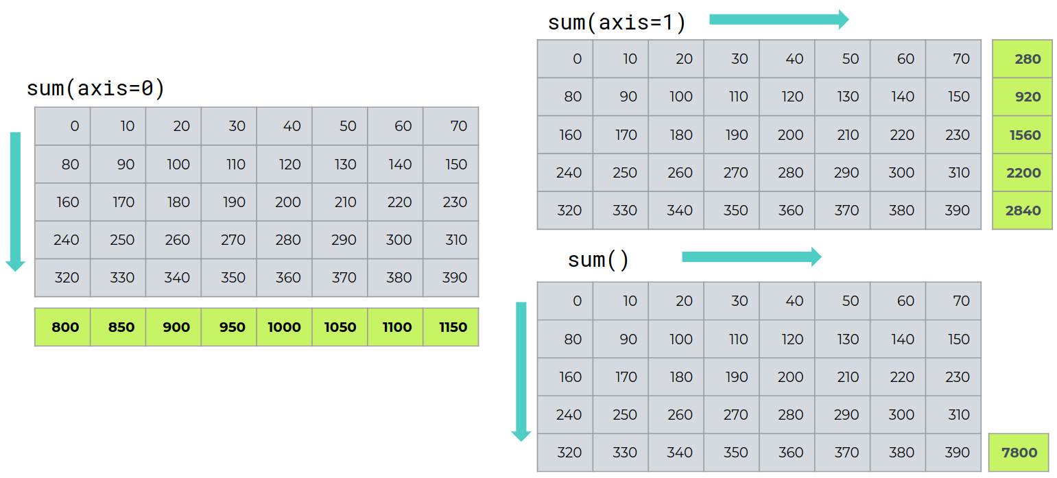
Reduction operations
Operations like sum, mean, max, ... are array reduction operations.
We call these reduction operations because operations like sum have the effect of slicing out n-D arrays from the input array, and reducing these n-D arrays to (n-m)-D arrays or scalars.
a=10.*np.arange(0, 40).reshape((5,8))
- mean:
a.mean() - std:
a.std() - sum:
a.sum() - min:
data.min() - ...
Rows sum
xprofile = data.sum(axis=0)
xprofile
Columns sum
yprofile = data.sum(axis=1)
np.allclose(xprofile.sum(), yprofile.sum())
xprofile.sum()
Floats comparison
Due to rounding errors, most floating-point numbers end up being slightly imprecise. As long as this imprecision stays small, it can usually be ignored. However, it also means that numbers expected to be equal (e.g. when calculating the same result through different correct methods) often differ slightly, and a simple equality test fails
a=0.15+0.15
b=0.1+0.2
a==b
numpy.allclose: use this function to compare arrays (or scalars)
If the following equation is element-wise True
then allclose returns True.
a=np.array([.5, 1., 1.05+0.45])
b=np.array([.5, 1., 1.+0.5])
a==b
np.allclose(a,b)
np.allclose?
Remove MODS bias
Load the MODS frame
with fits.open("data/mods1r.20171125.0026.fits") as hdulist:
    image = hdulist[0].data.astype(float)
NOTE: LUCI and MODS files have been downloaded from i2a archives in Trieste.
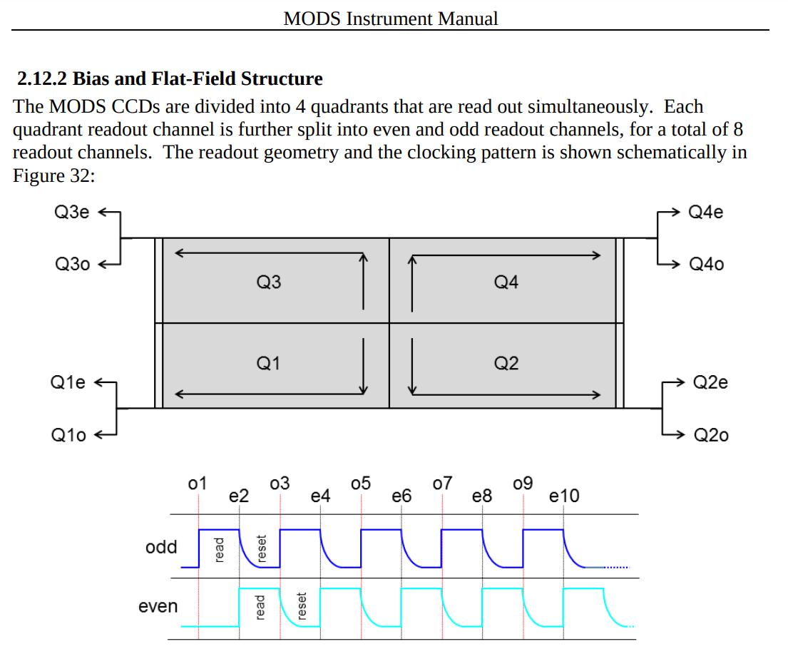
Quadrants and prescan regions
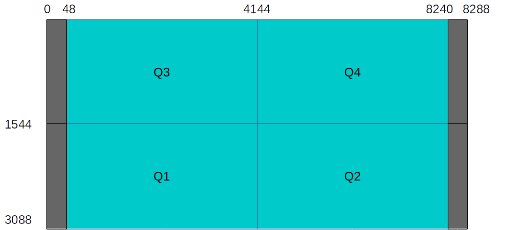
quadrants = [image[:3088//2,:8288//2],
             image[:3088//2,8288//2:],
             image[3088//2:,:8288//2],
             image[3088//2:,8288//2:]]
prscans = [image[:3088//2,:48],
           image[:3088//2,-48:],
           image[3088//2:,:48],
           image[3088//2:,-48:]]
Single prescan/overscan region
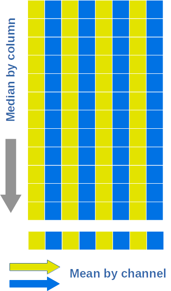
For each prescan region, we compute the bias level following this recipe:
- we compute the median levels along columns of the prescan region
- we compute to separated means: for even and odd channels.
8 Bias levels
Here we compute the bias level for each channel and remove these levels from image
from astropy import stats

for i in range(4):
  med = np.median(prscans[i], axis=0)
  bias_even = stats.sigma_clip(med[::2], sigma=2.0, maxiters=4)
  bias_odd = stats.sigma_clip(med[1::2], sigma=2.0, maxiters=4)

  quadrants[i][:, ::2]-=bias_even.mean()
  quadrants[i][:, 1::2]-=bias_odd.mean()
fits.PrimaryHDU(data=image).writeto("tmp/bias_sub.fits", overwrite=True)
Stats
The astropy.stats package holds statistical functions or algorithms used in astronomy. While the scipy.stats and statsmodel packages contains a wide range of statistical tools, they are general-purpose packages and are missing some tools that are particularly useful or specific to astronomy. This package is intended to provide such functionality, but not to replace scipy.stats if its implementation satisfies astronomers’ needs.
Masked array
- masked arrays are arrays that may have missing or invalid entries.
- these arrays are implemented by the NumPy module
numpy.ma - can be used in image processing to mask outliers, bad pixels, cosmic
- in catalog columns to mark invalid or missing entries
- ...
Get data
a.data
Get mask
a.mask
data operations
sumno masked data (default)
a.sum()
sumall data
a.data.sum()
- apply numpy functions
np.log(a)
mask operations
- get no masked data
a[~a.mask]
- change mask
a.mask=[True, False, False]
- change mask assigning a vald value
a[0]=2
a